Portfolio Management - A Financial Approach - Part 4

Introduction

We have almost reached the end of our journey through an economic approach to the management of a projects portfolio.

In the first post of this series we introduced some statistical concepts useful to analyze and optimize the composition of a portfolio of projects. In particular, we have characterized projects as black boxes, which absorb resources and generate returns. 

In the second post of this series we have derived the concept and mathematical formulation of what is called the efficient frontier, for a simple portfolio made up of two projects.

In the third post we explored a little more in depth the meaning of the the efficient frontier, analyzing its utility and how to use it to manage portfolio in a more effective way.  we sticked to the hypothesis of  a simple 2 projects portfolio as well.

In this post we will remove the hypothesis of  a simple 2 projects portfolio and we will expand what we have seen up to here to a generic portfolio made up of an arbitrary number of projects. We will see what implications this will have on our computational and graphical capabilities.

In the end we will introduce a kind of guide for a step-by-step implementation of the proposed approach.

The N-projects portfolio equations

In Figure 1 we can find the average return and average return standard deviation equations as derived in the second post of this series for the two projects portfolio.

Figure 1.

In Figure 2 we can see an extension of these equations for a N-projects portfolio. They are just a little bit more complicated that those depicted in Figure 1 but the rationale remains almost the same. The average return equation is still a linear combination of the average returns of the projects belonging to the portfolio. The average return standard deviation equation is a little bit more complicated, since all the covariances between one project and the others have to be taken into account. 

Figure 2.

At the end of the post I linked a presentation containing two different notations for the N-projects portfolio equations. These are the notations that we could probably find on math textbooks, but they are absolutely equivalent to the notation in Figure 2.

Clearly, the more projects we add to our portfolio the more a manual evaluation of the equations become unmanageable. Nevertheless, the appeal of this approach lies in the ease of implementation, since the equation presented can be easily implemented in a spreadsheet or in any high level programming language.

Some drawbacks

The first drawback we encounter is that with more than a few project, we completely lose the ability to represent effectively the efficient frontier on a graph. That is why I introduced the topic under the hypothesis of a portfolio made up of just two projects and I have stressed a lot the geometrical approach. At this point, having a clear understanding of the meaning of the equations, a multidimensional extension of the theoretical approach should be straightforward. It should be easy to manage and interpret the presented equations also in a multi-project environment, without a graphical aid.

The second drawback is that the more our portfolio becomes big, the more an evaluation of the efficient frontier's equations become computational intensive. As I have previously said, the method is easy to implement, nevertheless with many projects it quickly becomes computational intensive.

Please remember that the equations in Figure 2 have to be evaluated for each split of the budget between the projects that make up the portfolio. Here comes in our help what we have said in the last post of this series about the quantization of data. We are not dealing with portfolios of securities and we are not allowed to split the budget as we like. Each project could have just a few levels of expenditure and, as a result, the number of equations to be evaluated would fall significantly.

Implementation guide

1. Try to reduce each project to a kind of black box, that is, try to describe it as a function of the absorbed resources (money, people, materials...)  and of the generated benefits (money, services...). Evaluate each project’s average return and return standard deviation, as discussed in the first post of this series.
2. Evaluate the covariance between all the considered projects.
3. Evaluate the efficient frontier's equations for all the possible combination of budget allocations.
4. Select the budget split and the portfolio composition to achieve the desired average return or standard deviation. 
5. Pay attention not to be on a unfavorable zone of the efficient frontier, as we have seen in the third post of this series. Unfortunately we cannot afford the luxury of a graphic comparison. So attention must be paid on
• No other available budget allocation can generate a more profitable portfolio composition, in term of greater average return or lower uncertainty. That is, the portfolio composition is not on the red part of the efficient frontier, as shown on Figure 2 of the third post of this series.
• Slightly changing the portfolio composition (also trying combinations that are not actually possible) there is no possibility to achieve an increase of the differential average return greater than the differential uncertainty increase. That is, the portfolio composition is not on the orange part of the efficient frontier, as shown on Figure 3 of the second post of this series.

So, we have reached the end of our journey. I hope you have found this series interesting and useful. Please feel free to contact me for further details, comments, advices... 

N project portfolio from pmcrumbs

Quest' opera è distribuita con licenza Creative Commons Attribuzione - Non commerciale - Non opere derivate 3.0 Unported.

Portfolio Management - A Financial Approach - Part 3

Introduction

In the first post of this series we introduced some statistical concepts, useful to analyze and optimize the composition of a portfolio of projects. In particular, we have characterized projects as black boxes, which absorb resources and generate returns. 

In the second post of this series we have derived the concept and mathematical formulation of what is called the efficient frontier, for a simple portfolio made up of two projects.

In this post we will explore a little more in depth the meaning of the the efficient frontier, analyzing its utility and how to use it to manage portfolio in a more effective way. 

For sake of simplicity, we will stick to the hypothesis of  a simple 2 projects portfolio a little while yet.

The efficient frontier - What is this function telling us?

In Figure 1 we can see an example of efficient frontier for a 2 project portfolio. The reference equations are derived and explained in the second post of this series.

Figure 1.

Each point of the curve depicted in Figure 1 represents a particular split of the portfolio's budget, that is, the percentage of budget invested in project 1 and in project 2. The efficient frontier assigns to each budget subdivision and hence to each portfolio's composition, values of average return and return’s uncertainty.

It is therefore possible to decide a budget subdivision between the 2 projects and check the so obtained portfolio's average return and standard deviation. 

The other way round is also possible, we can choose a budget subdivision between the two projects to get a desiderable  average return, trying to remain inside defined range of return’s standard deviation.

A fundamental characteristic of the efficient frontier is that there is no better possible budget allocation, in the sense that, considering the projects at hand, we could not obtain a portfolio with a higher average return and a lower or equal standard deviation not residing on the frontier itself.

Figure 2.

On what part of the efficient frontier we would like our portfolio to be?

In Figure 2 we have split the efficient frontier in three parts. Remember that each point of the efficient frontier is a budget subdivision among the projects that compose the portfolio, to which are associated an overall average return and a return’s standard deviation.

• Red zone (A - B) Whatever happens, it is important to try to avoid this zone. As it is clearly depicted in Figure 1 and Figure 2, it is possible to find points on the Orange zone or Green zone with a greater average return and an equal return’s standard deviation. That is to say, there are ways to split the budget among projects that can lead to a greater average return with the same uncertainty.
• Orange zone (B - C) In this zone it is easy to see that the average return grows faster than the associated standard deviation. That is to say, moving from B toward C, we could achieve increases for the average returns that are greater than the increases of the associated uncertainty. So, even if it is not possible to find budget's subdivisions that lead to more efficient portfolio composition (greater average returns with equal or smaller uncertainty), it could be a good idea move toward the Green zone. A mathematical way to view the same concept is to find the place where the first derivative of the efficient frontier with respect to the return’s standard deviation gets smaller than 1. 
• Green zone (C - D) This is the better zone of the efficient frontier and possibly where a portfolio should be placed.

The effect of covariance on the efficient frontier

The covariance of the projects that compose the portfolio have an important effect on the efficient frontier's shape and position, as we can see In Figure 3. In the example the covariance between the 2 projects varies from 0 to +5 with unitary steps. The more the covariance increases, the more the efficient frontier moves towards the right of the axes. That is to say, we have to accept bigger risks to get the same average return. This is correct, because both the projects tend to go bad or well together. This leaves the average return more or less unchanged but it affects the associated uncertainty, spreading its magnitude.

Figure 3.

So it is clear that if we want to build a coherent and harmonized portfolio, the projects' covariances can be a very important resource, since they can be appropriately mixed to modulate the uncertainty associated to the portfolio's average return.

Where can we stay on the efficient frontier?

The theory here explained, had been originally developed to analyze and manage securities portfolios, where every budget partition is theoretically allowed. This leads to the fact that the efficient frontier is often represented as a continuous function and that should be possible to place a portfolio on each one of its points. On the contrary, projects' investments are often quantized. This constrains a projects portfolio to stay on just some points of the efficient frontier. 

As an example, we could diminsh the investment in a project from 120000 to 100000 dollars changing the quality requirements of some deliverables, but there could be no way to invest less than 100000 dollars or an amount of money between 100000 and 120000 dollars.

Figure 4.

In Figure 4 we can see how a quantized efficient frontier looks like. In this case we could be able to place our portfolio just on the coloured dots. That could be seen as a limitation right now but it will help us later, when we will remove the 2 projects hypothesis.

In the next post we will remove the 2 projects hypothesis and we will apply what we have seen until now to a generic N-projects portfolio. 

Quest' opera è distribuita con licenza Creative Commons Attribuzione - Non commerciale - Non opere derivate 3.0 Unported.

Portfolio Management - A Financial Approach - Part 2

Introduction

In the last post of this series, we introduced some statistical concepts useful to analyze and to optimize the composition of a portfolio of projects. In particular, we have characterized projects as black boxes, which absorb resources and generate returns. 
The returns were expressed in the form of a probability density functions, which are easily obtainable through Monte Carlo simulations applied to high-level planning of projects.
As a consequence, the only variables of interest to characterize a portfolio, are the average returns of projects and their associated standard deviations. The returns tell us how much projects are profitable on average, the variances tells us how much the average returns are uncertain.
Another measure, introduced in the last post and which will be extensively used here, is the covariance. That is, a quantity, dimensionally identical to the variance, which indicates the mutual behavior of two random variables.

In this post, we will see how to describe a generic projects portfolio's average profitability as a function of the associated uncertainty, starting from its composition and considering, for each project in the portfolio, the notions of average return, return's standard deviation and covariance.

The concepts presented in this post are largely derived from modern portfolio management theories introduced by Harry Markowitz and other economists, beginning from the first part of the ‘50s. 
For a full theoretic comprehension I recommend you to take a look at the two articles listed below.

• Harry Markowitz - Portfolio Selection - The Journal of Finance, Vol.7, No.1, Mar.1952
• Robert C. Merton - An Analytic Derivation of the Efficient Portfolio Frontier - The Journal of Financial and Quantitative Analysis, Vol.7, No.4, Sep.1972

Since the mathematic used in these articles is a little bit complex, especially if you do not have an engineering background, I will provide a simple explanation in the next part of the post. The articles are mainly focused on the selection of efficient portfolios of securities, considering interest rates and volatility. We will apply the same theoretical background in project portfolios management applications.

Two Project Portfolio Example

Let’s start considering, for sake of simplicity, a simple two projects portfolio. This can be done without infringing any generalities and will allow us to have a very straightforward discussion about the topic at hand, with the aid of simple graphic examples. The two project  constraint will be removed in subsequent posts of this series.

Figure 1.

Take a look at the first part of Figure 1. Let’s define some reference variables for each project and for the resultant portfolio. Return PDF is the return probability density function (PDF) as defined in the last post. Average Return and Return Standard Deviation are the mean value and the standard deviation of the PDF (so they are the mean return and the associated uncertainty) while Projects Covariance is the covariance between project 1 and 2.
Budget Percentual is the percentual that one invests in each project and, as a consequence, 1 is the percentual invested in the current portfolio. Boundary Condition accounts for this preposition.
As an example, if one whishes to invest 100000 dollars in the portfolio and x1=0.635, this means that 63500 dollars will be invested in project 1 and 36500 (x2=1-x1=0.365) dollars will be invested in project 2.

In the second part of Figure 1 we find some Equations. Equation (a) is the return of the current portfolio, evaluated as a linear combination of the returns of project 1 and project 2. This variable is a PDF, being a linear combination of probability density functions. Equation (b) is the average return of the portfolio. Equation (c) is the variance of the portfolio’s return. At the bottom of the post you will find a series of slides that explain how to get equations (b) and (c) starting from equation (a). I did not post the slides here to avoid encumbering the discussion.

Equations (b) and (c) are functions of two variables but, since the boundary condition that we discussed before, they can be described as functions of single variable. 
Since the summation of x1 and x2 must equal 1, one of the two variables could be substitued with 1 minus the other one's value. So, after having fixed a value for x1, we can substitute x2 with 1-x1. After this change, equation (b) and (c) of Figure 1 become the new equations (b2) and (c2) in Figure 2.

Figure 2.

In this new form they can be easily plotted on a bidimensional graph, as the one depicted in Figure 3. On the left we have a plot of the average return of the portfolio (equation (b2) of Figure 2) against the budget's percentual invested in project 1, while on the right we can see the portfolio return's variance (equation (c2) of Figure 2) plotted against the same variable.

Figure 3.

How can we use this 2 graphs? It is quite simple. We have to choose a budget's percentual to invest in Project 1 and read on the y-axis of the two graphs the expected portfolio return and its variance.

However this has two drawbacks. It forces us to look at two graphs to gather the information we need and the variance has a different unit of measure than the average. Since equations (b2) and (c2) on Figure 2 share the same domain, being both of them defined as a function of the percentual of budget invested in project 1, they can be plotted one against the other on a single graph, as the one presented in in Figure 4. We also take the root square of the return's variance, obtaining the return's standard deviation, that has the same unit of measure of the average return.

Figure 4.

Finally, on Figure 4, we see what is called the efficient frontier of the given portfolio. That is to say, the locus of point of maximal efficiency for the portfolio.
The utilization of this graph is straightforward. As an example, we can decide a portfolio’s average return, check the associated standard deviation and see how to split the available budget between the 2 projects. We will be sure that there would be no better allocation, in the sense that, considering the projects at hand, we could not obtain a portfolio with a higher return and a lower or equal associated standard deviation.

In the next post we will reprise the discussion from the efficient portfolio frontier and we will go a little more in depth on its utilization and interpretation. 

Quest' opera è distribuita con licenza Creative Commons Attribuzione - Non commerciale - Non opere derivate 3.0 Unported.

Portfolio Management - A Financial Approach - Part 1

Introduction

Sometimes it is not just enough do projects right. Sometimes It is compelling do the right projects. 

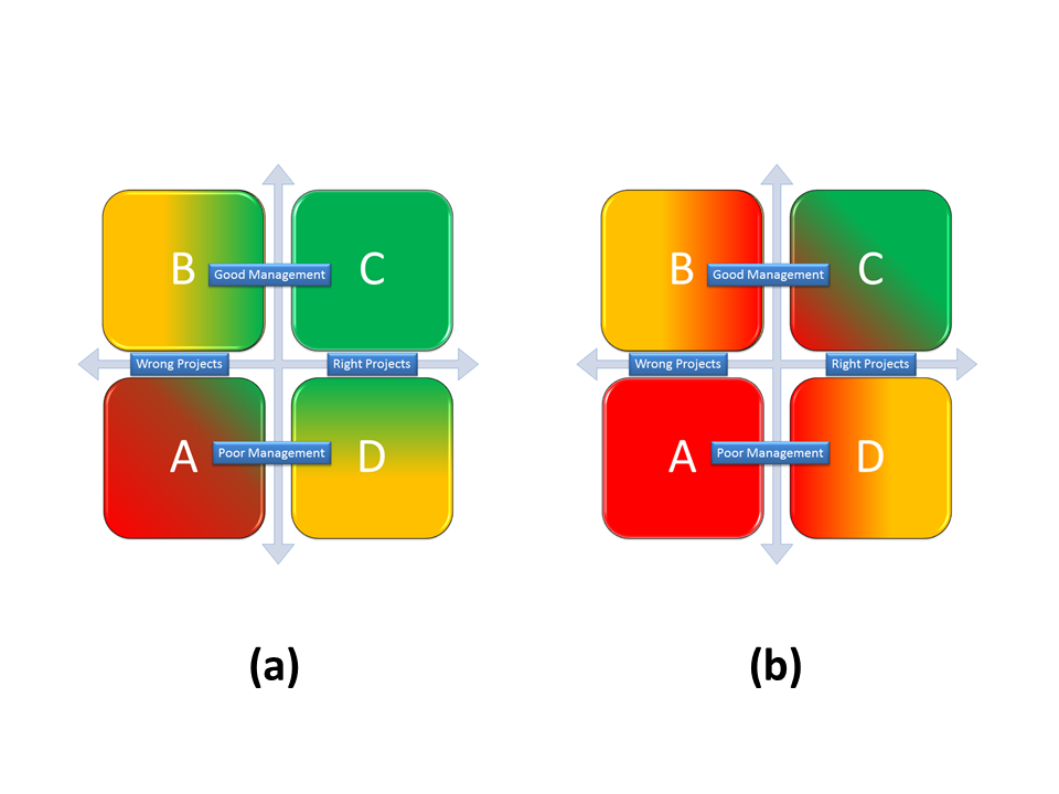
Let’s summarize on a graphic this affirmation. Take a look at Figure 1. On the x axis we can find the presence of appropriate or inappropriate projects in the portfolio and on the y axis the quality of the related project management activities. The graphic can be splitted in four quadrants.

Figure 1.

A - High expense and low income This is clearly the worst situation where one can be. Not appropriate and poorly managed projects. The portfolio suffer from a waste of resources due to poor management activities and from low income due to selection of inadequate projects.

B - Low expense and low income Wrong projects but managed well enough to contain the losses.

C - Low expense and high income This is the best situation. projects accurately selected and managed with reliable processes. 

D - High expense and high income Here the portfolio still suffer from a waste of resources due to poor management activities but it can count on high incomes due to a good projects selection.

It is generally true that everyone’s objective should be to create a portfolio placed in the C quadrant but in times of economic and financial downturn, this may become a matter of pure survival. Please take a look at Figure 2. In part (a), where the weather is fine and the sun shines on your economic situation, you can take the risk to fire some blank cartridges. This is not recommended but there is room for taking additional risks and make some wrong decisions.  when the rain comes in, as depicted in part (b), that it is no more an opportunity and when the mud starts to hit the fan, you are compelled to do better (better projects) with less (better project management). Even a portfolio placed in the quadrant C could not be safe and remunerative enough.

Figure 2.

So how to choose worthy projects to build a portfolio or better, how to choose projects more appropriate for given enterprise environmental factors?

There is a lot in literature about project selection methodologies. In these series of posts I will suggest a method based on some financial considerations. In this and other posts of the series there will be occasional references to statistical elements and concepts. I won’t explain in details each one of them (otherwise I probably would end up with an encyclopedia...) I will provide instead some reference links the first time each concepts is introduced.

Return estimation of a single project

Think of each project like a kind black box. You do not have the slightest idea of what happens inside them, you just know that they absorb resources (money, people, materials...) and that will generate (hopefully) benefits (money, services...).

Return: mean and standard deviation

The first step is to evaluate each project return as the difference of the expected benefits and the required investments, divided by the required investments. All the elements in the ratio should be reconducted to present discounted values. 

Figure 3.

The more you will be able to translate resources and benefits into money, the better you will be able to evaluate the project’s return.

Since the evaluation is based on economic projections and on high level project planning, the best way to do it is to derive a return PDF (Probability Density Function) with the aid of statistical techniques, like Monte Carlo simulations. In Figure 3 is reported an example of return PDF for a fictional project. A PDF is an analytic function that associates to a value on the x axis (in this case the project return) its probability density of occurrence. As an example, according to the return PDF depicted in Figure 3, there is a probability around 8% to achieve a return around 2% from the project. I used the word "around" and not "equal" given the subtle difference between continuous and discrete PDFs.

At this point it is possible, starting from the return PDF, evaluate for each project the mean return value and its standard deviation, that can be directly associated with the estimation uncertainty and with the project’s risk.

In Table 1 depicted in Figure 4 there is a representation of the previous evaluations for some fictional projects.

Figure 4.

Return covariance

The more the covariance of two random variables is great in absolute value, the more these two variables tend to change toghether. That is, if two random variables show great covariance in absolute value, when one of the two variables changes its value, the other one changes it with high probability. If two random variables show small covariance in absolute value, when one of the two variables changes its value, the other one is not bound to change with high probability. If the covariance is equal to zero then the two random variables are independent, that is to say that the behavior of one of them does not influence the other one.

The sign of the covariance shows if two random variables change accordingly. That is, a positive covariance states that two random variables assume great or small values together. A negative covariance states that while one of the two random variables increases (or lessens) its value, the other one lessens (or increases) it. The situation is summarized in Figure 4 Table 2, considering two random variables named x and y. The relationship is symmetric even if, for sake of simplicity, just one part of it is showed.

Assuming the return of each project as a random variable, the estimation of the covariance between each couple of projects is fundamental to properly set up a project portfolio, because it is important to know how the success or the failure of each project could affect the entire portfolio performance. 

Just to make a simple example, if a portfolio contains many projects that show a high degree of positive covariance,  a single project failure could severely affects the performance of the entire portfolio or, vice versa, a single project success could boost the entire portfolio’s return.

In the next post we will see how to select projects that shall be included in a given portfolio given a risk/uncertainty profile, using the statistical concepts here exposed.

Quest' opera è distribuita con licenza Creative Commons Attribuzione - Non commerciale - Non opere derivate 3.0 Unported.

Output, Outcome and Benefit - Managing today to shape the future

One of the most interesting and fascinating themes in Prince2 project management approach is, for what I am concerned, the business case one.

I find extremely interesting the constant focus on the project's business case and the continued assessment of the project justification, viability, and sustainability.

Also, I have been so impressed by the distinction between Output, Outcome, and Benefit.

Figure 1.

Output Each specialist product that the project has to deliver, be it tangible or intangible. Outputs are commonly delivered after the project’s closure and sometimes even during the project’s life.

Outcome Results of the changes derived from the use of the project's specialist outputs by the users. Outcomes typically start to be achieved after the handover of the project's specialist products to users.

Benefit Measurable improvement resulting from an Outcome. If the outcome is perceived as a disadvantage, we are dealing with what is called a dis-benefit. Benefits generally start to be achieved after the Outcomes and (should) continue to be achieved for a time span planned in advance. Prince2 states the establishment of a specific plan that describes the methods and times to verify the achievement of the expected benefits.

In Figure 2 we can see a quantitative representation of the relationship between these three ideas. Obviously, the exact Outcomes/Benefits realization times heavily depend on the project’s characteristics and peculiarity. 

Figure 2.

Let’s make a simple example to better clarify this view.

The Buymybooks Limited is a small company that sells books via the internet. Orders are collected by means of their internet site but after the initial collecting phase, orders are printed and processed manually. Also, Buymybooks Limited does not have a software to manage its books warehouse.

Their sell and delivery processes are highly inefficient, resulting in delivery errors, high costs, high customers turnover, and progressive reduction in the market share.

To face this situation, the board of director has decided to introduce a management software system to manage the sale and delivery processes.

Output of the project will be an integrated software management system (orders and warehouse management). 

Outcome of the project will be an improvement of Buymybooks Limited sell and delivery processes efficiency.

Benefits of the project will be delivery errors reduction, smaller costs, higher profits and greater customers' fidelity.

So we can agree that there is need to pay a great deal of attention not only to the execution phase of a project but also to the design, support and closure phases. Furthermore, it is of utmost importance check the actual realization of benefits after the project closure. This action should be performed by program or corporate management as prescribed in the project’s documentation. 

As a consequence, I would advise to

1) Have a series of compatible and well-crafted benefits

This seems obvious, but it can be sometimes tricky. I have covered the topic in one old post. It has been conceived for project objectives, but it is well suited for project benefits too.

2) Do not just focus on the outputs delivery

Sometimes, is easy to focus just on output delivery and lose contact with project’s outcomes and benefits. It could happen if outputs are the only substantial point of contacts between the project and the team members (that sometimes ignore the big picture), or between the project and the external stakeholders. 

Also, it is not uncommon to rely just on outputs delivery to measure project’s completion or success.

3) Choose the best possible approach to maximize benefits

Since a significant part of the project’s value will be realized after project’s closure, take care, during project planning, in choosing the best possible project approach to maximize the expected benefits and not just the outputs production. 

In the same way, while drafting the business case, do not take into account just the specialist products realization and delivery costs. Keep an eye also on handover, maintenance and operational costs. 

Manage and execute the project thinking also to the desired outcomes and benefits, trying to increase the probability of success and to maximize their impact on business as usual. 

4) Close a project if it has been proved to be no more justified, viable and sustainable

A project is a mean to reach an objective and not an objective in itself. Stop investing in a project if it is not longer worth it, is not a failure. Honor to the project manager who conscientiously proposes an early closure of its project, out of respect for the corporate vision.

Keep on throwing money out of the window. That surely is a failure.

To keep track of some of this aspects, I suggest the use of two very simple tools.

benefits/benefits matrix (Useful for points 1 and 4)

The first one is a matrix on which all project benefits are listed in columns and rows, sorted by descending importance, from left to right and from top to bottom. Each benefit's importance is recorded near the benefit's code. You can find an example of the benefits/benefits matrix in Figure 3.

At the intersection of each row and column of the matrix, there is a symbol that explains the benefit's relationships. 

Figure 3.

The “+” sign represents a high degree of correlation between two benefits' viability. This bond leads to risky situations because there is a high probability to realize both the benefits (opportunity) or to miss them both (threat). 

The “-” sign accounts for a low consistency between two benefits. This bond leads to risky situations because the realization of one of the two benefit could jeopardize the achievability of the other one.
In the example depicted in Figure 3, the achievability of benefits B2 and B3 is correlated. Benefits B1 and B4 are not consistent, but the real problem is that benefits B2 and B4 are not consistent too and, as a consequence, also benefit B3 is jeopardized. So benefit B4 jeopardizes benefits B2 and B3, that are the most significant benefits of our project.

Especially if one or both the benefits are assessed as paramount, strong “+” or “-” relationships have to be dealt with the greatest attention by the project manager. 

if too much “+” and/or “-” relationships appear in the benefits/benefits matrix, it could be wiser TO conduct an additional analysis of the project's expected benefits and to reassess the project’s riskiness. 

If two benefits do not have specific relationships, the intersection between their columns and lines is left empty. Obviously, the matrix is symmetric by construction and the slashes on the main diagonal are inserted just for the sake of clarity.

Other symbols could be added to account for different relationships, even if I advise to keep things as simple as possible.

Even in this very simple form, this tool could help in identifying dangerous (-) or risky situations (+), and contribute to the definition of the project's objectives.

products/benefits matrix (Useful for points 2 and 3)

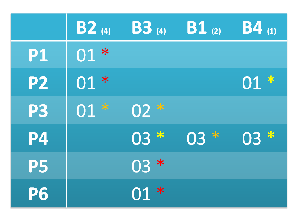
The second tool I want to present is a matrix on which all project products (outputs) are listed in rows and all project benefits are listed in columns. Benefits are sorted by descending importance from left to right. Each benefit’s importance is recorded near the benefit's code. You can find an example of the products/benefits matrix in Figure 4.

Figure 4.

Each intersection between a row (product) and a column (benefit) contains project's outcome's codes, and represents through which outcome a single product helps to achieve a benefit. The color code states the degree of importance of the product to the expected benefit's realization (e.g., red could mean high, orange average, and yellow low).

We can see, reading the matrix by columns, which product helps to achieve a benefit, and to which degree each product is necessary to this end.

In this way, we can maintain a constant focus not only on project’s outputs but also on project’s benefits, through project’s outcomes.

If we are forced to drop out a product, we can immediately see which benefits are at stake, their importance for the project and how much they are at risk. It is a simple way to depict the effect of a project scope modification on the project benefits.

In the same way, if we decide to sacrifice a benefit, we can immediately evaluate if there should also be a project’s scope modification.

If you feel like to read some suggestion on how to assign importance values to project benefits, please refer to this post. It has been conceived to suggest how to assign qualitative values of impact and probability to project risks, but I think that the content is perfectly adaptable to the current problem.

Quest' opera è distribuita con licenza Creative Commons Attribuzione - Non commerciale - Non opere derivate 3.0 Unported.

Are your project objectives S.M.A.R.T. enough?

I love acronyms.

I have always considered acronyms as incredibly shrewd and useful tools, for communicating and for remembering complex concepts in a simple and effective way.

In this post i will focus on one acronym that I came across the first time while studying Prince2 and that, as often happens, I then met again several times in the following days, even if slightly modified.

The acronym is S.M.A.R.T. and, related to project objectives, stands for Specific, Measurable, Achievable, Realistic, and Time Bound.

Honestly, I have to say that there seems to be no universal agreement on the words whose initials make up this acronym, as you can see by following this link. However, the version presented here is the one that I find more congenial and useful to my needs.

Specific

How could you hit a target, if you do not know where the target is? Or worst, how could you hit it, if you do not even know what the target looks like? In the same way you cannot achieve a objective if you do not provide (or if you have not been provided with) a clear description of the objective itself.

It seems obvious, I think that everyone would agree with the previous statement...but please keep in mind that defining specific objectives for a project is not an easy task.

To state or analyze a clear and well crafted business case, considering all present and future developments, benefits and advantages, requires both great project insight and business vision. You could need the aid of a business analyst and, possibly, great support from your corporate management.

If you have been provided with project documentation, in the form of a charter or of a project brief, take your time to examine it carefully and request clarifications wherever necessary.

Never get tired to inquiring your project's documents because, you know, the devil is in the details.

I believe that not to specify clearly project objectives is not a smart (and obviously not a S.M.A.R.T.) shortcut but the highway to failure.

Measurable

All the objectives must be measurable. Period. Always. Period.

If you do not have measurable objectives, it will be impossible to determine if you have been successful or not. It will also be impossible to determine the degree to which the project has fulfilled its expectations.

Also as you might rationally decide to terminate or to continue the project, if you do not have precise targets to measure progress? How could you reassess  the business case? This could result in a massive expenditure of money without proper justification. Also, if you haven’t properly quantified your objectives, it is consequently impossible to determine their risk exposition and, as a consequence, it is impossible to determine the project’s risk exposition. No good. Believe me. 

The problem here is to find proper ways to measure objectives.

Even this one can be a daunting task, depending on the particular industry you are in.

It is easy to measure the number of defective pieces of equipment coming out from a production line, or the lifetime of a new electric bulb. It is more difficult when it comes to customer satisfaction, software quality, reputation improvement, products quality improvement...In these cases an indirect measure could do the job.

As an example you could measure the number of contacts of your customer service  and put it in relation with an improvement or a worsening of your products.

The bottom line is: everything can be measured, the problem is to identify suitable measurement units. It is a complex problem but is a problem that can be and must be solved.

Achievable

Some objectives just do not go well together. They seem to live in orthogonal dimensions.

Sometimes it seems that a complete scope, a fast time to market, a low budget and an high quality standards mix well...as oil and water.

So take care in having an achievable and consistent set of objectives. If it is not the case, try to reconcile reality with management's desires and expectations.

Never start a project that has not achievable objectives, pretending that everything is just fine and thinking ahead how to justify the unavoidable failure or below average performance.

Realistic

Everyone would like to be in charge of the next multi-billion dollars, thousands resources, hundred contracts project, with all the whistles and bells. Reality is, many times, different. 

The project manager’s duty is to reconcile budget, time, scope, quality and all the other constraints into a shared and satisfying vision, be he/she in charge of a mega project or working in small businesses. The duties of a project manager toward the sponsor and the stakeholders do not change with budget’s size. Again, he/she must reconcile reality with management desires and expectations and must resist the temptation to artificially raise the bar in order to magnify its own role.

Time Bound

Every project should have a starting date and an ending date. Every objective should be achieved in the defined timeframe. Benefits could be achieved later on but a time span have to be defined as well.

This is an important commitment for a project manager.

So there is no point in defining objectives that cannot be achieved in the project timeframe or in the expected time for benefits realization, once project products are released in the operation environment.

Otherwise, an attitude of this kind could frustrate team members, create distrust in corporate management and alienate stakeholders. 

Quest' opera è distribuita con licenza Creative Commons Attribuzione - Non commerciale - Non opere derivate 3.0 Unported.

Assumptions and data: never get tired to question them

Let me play a little game with you, just to introduce the subject of this post.

Solve this very easy riddle. 

“Hi, 

I am a very big mammal. 

I am an herbivorous.

I have a grey thick skin.

You can find me in Africa but I have cousins in Asia.

I have been (and I am still) hunted by humans because of something that grows near my mouth.

Who am I?

If you want to meet me follow the link.”

Are you surprised?

Did you expect to meet this other African friend?

Well...you are not totally wrong...or more precisely...you are right...too.

From the data at your disposal both the answers were right. Both these animals are big herbivorous mammals with a grey thick skin. Both of them are present in Asia and have been hunted almost to extinction because of something that grows on their muzzle...and yes...nose and mouth are quite near.

Almost everyone indicates the elephant as a solution for this riddle, probably because elephants are more ubiquitous than rhinos on television, cartoons, books, tales...

What your brain does

The fact is that you have been provided with true but incomplete data and your brain automatically tried to fill the gaps in the best way it could. It tried to interpolate data where informations were lacking.

This capability is something wonderful and amazing at the same time. Your brain, starting from some provided data and past stored knowledge, suggests you answers when you have to take decisions. This same capability is what comes at your help when you have to make an educated guess about some event in the future.

I value this as one of the most important characteristics of human beings.

Take it easy

Please, do not have fear, in this specific case is not your brain that have deceived you...but the other way round...you probably have not provided him with enough time to give a well crafted answer to the riddle I proposed you.

Probably if you had waited a little, if you had just taken your time before trying to give the answer it would have come to your mind that the riddle would have been satisfied by at least two answers. The problem was that everything seemed so perfect, the data seemed so accurate, so precise that you jumped directly to your conclusion. 

This happens in day to day life and in project management too, whenever we have to deal with data and/or assumptions to take decisions.

Sometimes we trust too much the data we have been provided with or the assumptions we have accepted as true, especially when data seem so well crafted and our first answers seem to fit so magically...in this cases sometime we are driven to rush headlong to conclusions.

What we have to deal with

In Figure1 we can see a pictographic representation of a two dimensional data  space, where data and assumptions are placed using their degree of completeness and reliability. Above the yellow line we have data and assumptions more reliable than complete. This is the same situation we have faced with the riddle.

Below the yellow line we can find data and assumptions more complete than reliable.
Both situations are critical.

Figure1.

In the first situation efforts have to be made to collect more data and to refrain from giving the answer too quickly. Take your time. If it is too good to be true...probably it is not true. So try to collect fresh informations and evaluate alternatives to your decision.

In the second one efforts have to be made to verify and validate data and assumptions, discarding corrupted ones. The problem is...how do we know that our data are not reliable or our assumptions are fault? 

Well...the only answer I can offer is to never get tired to analyze, check, question and validate.

Always perform data and assumptions sanity checks, base your analysis on literature, consult with the team, consult with the stakeholders, consult with other project managers and with your project management office... Check lessons learned related to other similar projects if you can access them.

...So

Maintain these behaviors for all the project life. Never get tired to evaluate alternatives and to question and check your data and/or assumptions...or you run the risk to mistake an elephant with a rhino...or even worse...an assumption with a million dollars gamble. 

Thank you for reading.

Bye.

Quest' opera è distribuita con licenza Creative Commons Attribuzione - Non commerciale - Non opere derivate 3.0 Unported.

A very simple tool for portfolio analysis

In my post Is it time to go Agile ? I suggested to dispose projects in a bidimensional space, whose coordinates were Innovation and Complexity. This had been done in order to group projects in different classes and to identify for each one the most suitable project management approach.

Figure 1.

In this post I will expand further the concept of projects grouping but with a totally different goal.

The purpose here will be to evaluate reliable indicators to depict the levels of Innovation and Complexity of given portfolios and assess their coherence with the corporate’s profile and business objectives.

To do this we will dive a little in vector’s math to find a more appropriate representation of our bidimensional space.

As it is known a point in a cartesian plane can be unambiguously identified by mean of its two orthogonal projections on the cartesian axes, as shown in Figure 2.

Figure 2

Here the tuple of coordinates (a,b) unambiguously identify the point. This system is called cartesian coordinates system  and numeric values are found on the intersections between  the cartesian axes and the orthogonal lines traced from the given point.

This is not the only possible representation. In Figure 3 is shown the way a point can be unambiguously identified  in the same space by mean of a different set of coordinates. 

Figure 3.

This system is called polar coordinates system and a point is identified by its radius, the point’s distance from the cartesian axes intersection and its azimuth, the angle (positive counterclockwise) from the abscissa axis.

In Figure 3 are also depicted formulas to switch from a coordinates system to the other.

In Figure 4 are shown all possible values for radius and azimuth obtained assigning to Innovation and Complexity values taken from an integer number linear scale ranging from 1 to 6. 

Figure 4.

M (radius) is represented in absolute values while Phi (azimuth) in degrees from 0 to 90.

An overview on values assignement to projects attributes can be found on my post Risk qualitative analysis. How much complicated ?. 

Using polar coordinates the project space represented in Figure 1 looks like as shown in Figure 5.

Figure 5.

Each project is now depicted as a vector and is unambiguously identified by its radius and its azimuth.

An alternative representation for projects in a bidimensional space has been introduced, but was it worth it ? Two numbers we had before (a,b) and two numbers we have now (M, Phi). what is the worth of all this work ?

Figure 6.

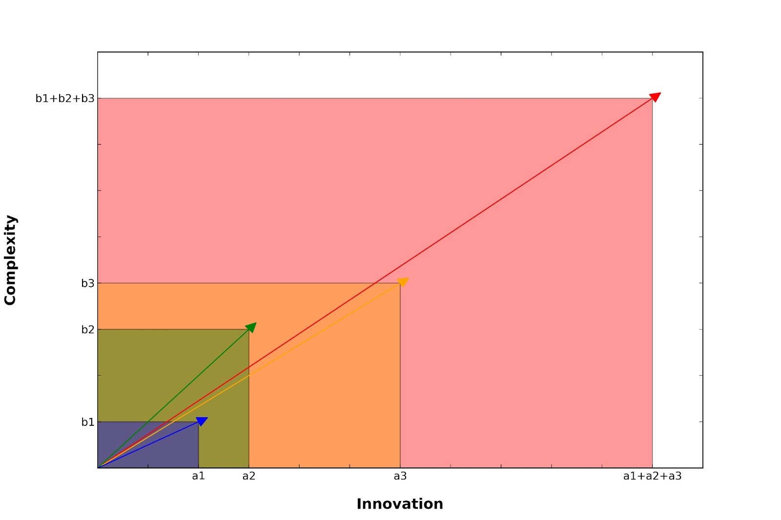
The answer to this question can be found on Figure 6. Observe how the sum operation works on vectors. The sum of N of vectors is still a vector, with abscissa and ordinate equal to the sums of abscissas and ordinates of the N vectors that have been summed together. In this example the red vector is the sum of the blue, yellow and green ones. Consequently the result of this operation depends both on vectors radius and azimuth, as can be observed in Figure 7. 

Figure 7.

Here three vectors with unitary radius are summed together in both the upper and in the lower part of the figure. Vectors in the lower part have a wider range of values for the azimuth coordinate and as a result their summation leads to a vector with a different azimuth and a shorter radius.

So we can say that the more two vectors are alike (radius and azimuth) the more the vector resultant from their summation has a greater radius coordinate. 

As a limit case, if all the 3 vectors in the example were equal in radius and azimuth, the summation result would have been a vector with a radius 3 times the original radius and an azimuth equal to the original one.

Following this line of thought we could add up all the project vectors in the bidimensional space and use the resultant vector as a portfolio indicator. Formulas are depicted in Figure 8.

Figure 8.

The radius value divided by the number of addenda assess how complex is a project in term of Innovation and Complexity, the azimuth how the portfolio is balanced toward the two coordinates. 

A low azimuth indicates that a Portfolio is balanced toward Innovation, a greater one that a Portfolio is balanced toward Complexity. In Figure 9 some examples can be seen. 

Here four portfolios are being analyzed using the suggested indicator. Portfolio in panel a has a lot of projects with an high degree of Complexity and with a medium grade of Innovation. As a result the indicator vector has a great radius and  azimuth values, stating its balance toward Complexity. Portfolio in panel b has some project with an high degree of Complexity and with a medium grade of Innovation and some project with a low degree Complexity and low grade Innovation. As a result the indicator vector has a medium values both for radius and azimuth. There is a balance here between 2 different classes of projects. The bunch of projects near to the ascissa axis counterbalance the high Complexity projects, even if it is clear that the portfolio is still polarized toward Complexity. 

Figure 9.

Portfolio in panels c and d are composed by projects with similar degrees of Complexity and Coherence but with very different balances. The indicator vector here reflects well the situation.

This approach is expandable toward an higher number of dimensions. In case it would support more complex analysis with more parameters, like the Uncertainty parameter proposed as a third dimension in my post “Is it time to go Agile?”. 

Property of Euclidean Space in fact holds for every number of dimensions even if, clearly, our graphical representation capability stops to three. The only price to pay is a little more sophisticated math, since in a K-dimensional space we would have K dimensions to sum together for radius evaluation and K-1 azimuth coordinates.

Quest' opera è distribuita con licenza Creative Commons Attribuzione - Non commerciale - Non opere derivate 3.0 Unported.