Portfolio Management - A Financial Approach - Part 1

Introduction

Sometimes it is not just enough do projects right. Sometimes It is compelling do the right projects. 

Let’s summarize on a graphic this affirmation. Take a look at Figure 1. On the x axis we can find the presence of appropriate or inappropriate projects in the portfolio and on the y axis the quality of the related project management activities. The graphic can be splitted in four quadrants.

Figure 1.

A - High expense and low income This is clearly the worst situation where one can be. Not appropriate and poorly managed projects. The portfolio suffer from a waste of resources due to poor management activities and from low income due to selection of inadequate projects.

B - Low expense and low income Wrong projects but managed well enough to contain the losses.

C - Low expense and high income This is the best situation. projects accurately selected and managed with reliable processes. 

D - High expense and high income Here the portfolio still suffer from a waste of resources due to poor management activities but it can count on high incomes due to a good projects selection.

It is generally true that everyone’s objective should be to create a portfolio placed in the C quadrant but in times of economic and financial downturn, this may become a matter of pure survival. Please take a look at Figure 2. In part (a), where the weather is fine and the sun shines on your economic situation, you can take the risk to fire some blank cartridges. This is not recommended but there is room for taking additional risks and make some wrong decisions.  when the rain comes in, as depicted in part (b), that it is no more an opportunity and when the mud starts to hit the fan, you are compelled to do better (better projects) with less (better project management). Even a portfolio placed in the quadrant C could not be safe and remunerative enough.

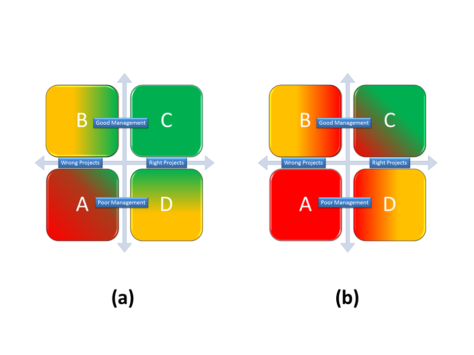
Figure 2.

So how to choose worthy projects to build a portfolio or better, how to choose projects more appropriate for given enterprise environmental factors?

There is a lot in literature about project selection methodologies. In these series of posts I will suggest a method based on some financial considerations. In this and other posts of the series there will be occasional references to statistical elements and concepts. I won’t explain in details each one of them (otherwise I probably would end up with an encyclopedia...) I will provide instead some reference links the first time each concepts is introduced.

Return estimation of a single project

Think of each project like a kind black box. You do not have the slightest idea of what happens inside them, you just know that they absorb resources (money, people, materials...) and that will generate (hopefully) benefits (money, services...).

Return: mean and standard deviation

The first step is to evaluate each project return as the difference of the expected benefits and the required investments, divided by the required investments. All the elements in the ratio should be reconducted to present discounted values. 

Figure 3.

The more you will be able to translate resources and benefits into money, the better you will be able to evaluate the project’s return.

Since the evaluation is based on economic projections and on high level project planning, the best way to do it is to derive a return PDF (Probability Density Function) with the aid of statistical techniques, like Monte Carlo simulations. In Figure 3 is reported an example of return PDF for a fictional project. A PDF is an analytic function that associates to a value on the x axis (in this case the project return) its probability density of occurrence. As an example, according to the return PDF depicted in Figure 3, there is a probability around 8% to achieve a return around 2% from the project. I used the word "around" and not "equal" given the subtle difference between continuous and discrete PDFs.

At this point it is possible, starting from the return PDF, evaluate for each project the mean return value and its standard deviation, that can be directly associated with the estimation uncertainty and with the project’s risk.

In Table 1 depicted in Figure 4 there is a representation of the previous evaluations for some fictional projects.

Figure 4.

Return covariance

The more the covariance of two random variables is great in absolute value, the more these two variables tend to change toghether. That is, if two random variables show great covariance in absolute value, when one of the two variables changes its value, the other one changes it with high probability. If two random variables show small covariance in absolute value, when one of the two variables changes its value, the other one is not bound to change with high probability. If the covariance is equal to zero then the two random variables are independent, that is to say that the behavior of one of them does not influence the other one.

The sign of the covariance shows if two random variables change accordingly. That is, a positive covariance states that two random variables assume great or small values together. A negative covariance states that while one of the two random variables increases (or lessens) its value, the other one lessens (or increases) it. The situation is summarized in Figure 4 Table 2, considering two random variables named x and y. The relationship is symmetric even if, for sake of simplicity, just one part of it is showed.

Assuming the return of each project as a random variable, the estimation of the covariance between each couple of projects is fundamental to properly set up a project portfolio, because it is important to know how the success or the failure of each project could affect the entire portfolio performance. 

Just to make a simple example, if a portfolio contains many projects that show a high degree of positive covariance,  a single project failure could severely affects the performance of the entire portfolio or, vice versa, a single project success could boost the entire portfolio’s return.

In the next post we will see how to select projects that shall be included in a given portfolio given a risk/uncertainty profile, using the statistical concepts here exposed.

Quest' opera è distribuita con licenza Creative Commons Attribuzione - Non commerciale - Non opere derivate 3.0 Unported.

Risk qualitative analysis. How much complicated ?

When it comes the time for risk qualitative analiysis, project manager and his team are required to express qualitative estimations of some risk attributes, tipically probability and impact, by means of subjective values or judgment.

These estimations are mainly based on project insight achieved by team members until that moment and some kind of a priori knowledge about the nature of the risks themselves.

Obviously the more these informations are reliable, the more this subjective qualitative analysis is trustworthy.

In the next of this post I will give some little tips that I think could ease this process.

Keep it simple

The objective is to have a simple and effective way to establish which risks worth a more specific quantitative analysis and which must be simply checked from time to time, rendering this information in a way that almost everyone can understand in a glimpse of an eye. 

So use simple indicators as numbers, letters or definitions. Don't use long wordy descriptions. These can find more suitable space in the risk description documents.

Figure 1. Simple is better...and understandable even after months.

Few Attributes

Two attributes are best. 

People normally find easy taking decisions based on two variables charts, conversely can be dismayed coping with multi-dimensional space. 

In figure 2 are represented a 2D scatterogram on the left  and a 4D scatterogram (colors are the fourth dimension) on the right. As we can see the scatterogram on the right is plenty of information but it is very difficult to understand. Conversely it is straightforward taking decisions based on the 2D graph.

I have seen indicator systems so complex and so difficult to read, that even the team who created them loosed the grip on their meaning after less than one month.

Probability and Impact are everything you need to know in this stage. 

Figure 2. On the left a 2D scatterogram. On the right a 4D scatterogram. The 4D graph is far richer of informations but it is difficult to understand.

Linearly spaced values

Logarithmic scales, Modified Fibonacci series, Repfigit numbers...well...are we still talking about project management or did we switch to astrophysics ? 

Methods mentioned above are surely useful in many ways but are also very difficult to familiarize with.

I think that for simple qualitative analysis nothing can be better than a plain old linear sequence.

Figure 3. Everyone can easily manage linearly spaced values.

Even integer numbers

Use even integer numbers every time you can. 

Decimal number are a useless complication. 1 to 10 in 0.1 step have the same meaning than 1 to 100 with step 1.

If you use odd numbers the mean is among possible values and this tend to polarize the estimation, you will end up using 3 more than the dued if you values are between 1 and 5. Guaranteed.

Take a look at Figure 4. 

I guess your attention has been dragged immediately to the middle, right ?

Now take a look at figure 5.

See how different is your perception ?

Using integer numbers you are every time compelled to make a choice. Under the mean or above the mean. No neutrality.

Figure 4. What are you looking at ? The one in the middle ? 

Figure 5. And now ? What are you looking at ? 

Few values

What is the point in having a scale that goes from 1 to 10 if people use 90% of the time values between 4 and 8 ? Too much values can be confusing. 

It is sometimes difficult to perceive and assess effectively an attribute value on a long scale based on subjective considerations only. Especially if the team is not accustomed to it or not extremely experienced.

In figure 6 we can see a 10 values bar chart on the left and a 4 values bar chart on the right. What is the difference between 7 and 8 or 8 and 9 ? Are you sure you can state it just basing your judgment on subjective data only ? Which graph is more intelligible ?

Two values are too little, four are best, six are even better if the team is experienced, eight are definitely too much. 

The only exception is if you intend to use values assigned to risk attributes during qualitative analysis to infer a suitable probability density function to be used in quantitative analysis, as I stated in my 12 November 2012 post A structured approach to qualitative risk analysis.
In this case you do need to use many values in your evaluation scale.

Figure 6. On the left a 10 values bar chart. On the right a 4 values bar chart. Which one is more intelligible ? What is the real difference between 7 and 8 and 9 ?

Standardize the values

2 is a number. It doesn't have a meaning by itself. You have to provide that meaning.

For example :

1. Risk impact less than 200000 USD
2. Risk impact between 200000 USD and 400000 USD
3. Risk impact between 400000 USD and 600000 USD
4. Risk impact above 600000 USD

Best is when the standardization is at a corporation level, so that every project manager and team member could immediately understand what is at stake.

Judgment or numbers ?

Sometimes number can intimidate people that could feel more at ease using judgment as Very low, Low, High, Very high. 
Still it is necessary  a standardization at a corporation level.

...In the end 

My point is that using a sequence like 1, 2, 3, 4 or 1, 2, 3, 4, 5, 6 should be best for risk qualitative analysis in most projects in most organizations and that you shouldn't consider more than two risk attributes at this stage. Any values you decide to use must be provided with a clear, unmistakable and standardized meaning at corporation level. 

Quest' opera è distribuita con licenza Creative Commons Attribuzione - Non commerciale - Non opere derivate 3.0 Unported.

A structured approach to qualitative risk analysis

Have you ever undergone the terrible experience of needing a plumber on Christmas day?
If your answer is "yes", you will have learned the hard way that the impact of a random event is a function of time. The same can be said about the probability.

So, when it comes the time for qualitative risk analysis, is rather a simplistic approach, assign constant values for risks' probability and impact, not considering the time dependency that these variables have.

Normally, qualitative risk analysis is a prelude to the quantitative one, in which a thorough risks review is carried out with appropriate statistical tools and methods.

Nevertheless, a structured approach for risks qualitative analysis could be helpful for projects which

• Are too small to justify both qualitative and quantitative risk analysis.
• Have so many risks, that performing a complete quantitative analysis could be too much time and resource consuming.

So, my suggestion is that every time a qualitative analysis is performed

• Assess probability and impact values for all the project risks, for the entire project life cycle. Do not assign constant values that are meaningful just for the here and now. Try to forecast future values and reasses past ones, expressing them as a function of time, using all the information you can get.
• Collect, analyze, and potentially correct all your previous estimations.

Please, take a look at the next two images.
The qualitative risk analysis of Risk #001 has been performed as a function of time and covers the expected project life cycle.

Figure 1 depicts the qualitative value assigned to the occurrence probability of the risk; figure 2 represents the qualitative value assigned to its impact.
Both values  are provided for the entire project time horizon and depicted as functions of time.

Figure 1: Probability as a function of time.

Figure 2: Impact as a function of time.

As we can see, a quantitative analysis of the current risk could be quite safely avoided until May. 

So, indications to perform quantitative risk analysis on risk #001 in Q2 can be added to the risk management plan. 

During project execution, if new evaluations would contradict the present data, risk #001 could immediately undergo the analysis process.

In figure 3 and figure 4 is shown the qualitative risk analysis temporal evolution for risk #001. 

Every 3 months the qualitative risk analysis results have been questioned in the light of new information, obtained during project execution, and the assessments of probability and impact corrected. 

The probability value has been set to zero for past months since the risk didn't occur.

The risk's impact value on the project has been instead reassessed also for past months. 

The reassessment process is useful for following reviews of the qualitative risk analysis effectiveness.

Figure 3: Probability as a function of time. Qualitative analysis performed each 3 months.

Figure 4: Impact a function of time. Qualitative analysis performed each 3 months.

In figure 5 it can be seen an estimation of the accuracy of the qualitative risk analysis performed on risk #001.
The horizontal lines represent the risk impact mean values of all the evaluations performed during the project life cycle (actual values can be seen in Figure 4) while the vertical lines depict the standard deviation values (mean +/- sigma). 

Figure 5: Impact. Means and standard deviations for each estimation as a function of time. 

The showed graphical representation can be very useful during project closure and lessons learned collection. Figure 5 shows how well (or how bad) we have performed qualitative risk analysis.
The presented approach helps project managers to understand how to refine estimations, and the degree of uncertainty it can be expected for similar projects.

Figure 6 and figure 7 depict the temporal evolution for the qualitative values of probability and impact for risk #001 (actual values can be seen in figure 3 and 4). 

Figure 6: Probability as a function of time for a single month estimation. Month is August. See also Figure 3. 

Figure 7: Impact as a function of time for a single month estimation. Month is September. See also Figure 4. 

It can be seen that for the selected months, the probability assessed value decays with a quadratic law while the impact value changes linearly.
Mathematical models and polynomial fitting techniques can be used to discover hidden patterns in the data, and the velocity of convergence of an estimation to an unbiased value. Results could also be correlated with previously conducted analysis and grouped by risks area.

The proposed approach could be useful in aiding project managers to refine their estimations for future projects, it could display the natural tendency to overestimate or underestimate particular categories of risk in particular moments of the project life cycle, and can be used to debias estimations, conducting to more reliable forecasts.

The bottom line is that having qualitative evaluations for each project risk in the form of time function can be helpful for

• Determine when a particular risk deserves a quantitative analysis, plan the required actions and allocates the required resources well before the task can become critical.
• Select a proper statistical probability distribution to be used in quantitative analysis and in statistical simulations. For example it could be estimated fitting a model over the curves presented in the first 2 figures.
• Allocate contingencies in a more effective way.
• Get debiased estimations and more reliable forecasts.
• Assess the qualitative risk analysis effectiveness and correctness.
• Estimate the natural tendency of a particular project manager in overestimating or overestimating particular categories of risk in particular moments of the project life cycle.

Quest' opera è distribuita con licenza Creative Commons Attribuzione - Non commerciale - Non opere derivate 3.0 Unported.