Portfolio Management - A Financial Approach - Part 4

Introduction

We have almost reached the end of our journey through an economic approach to the management of a projects portfolio.

In the first post of this series we introduced some statistical concepts useful to analyze and optimize the composition of a portfolio of projects. In particular, we have characterized projects as black boxes, which absorb resources and generate returns. 

In the second post of this series we have derived the concept and mathematical formulation of what is called the efficient frontier, for a simple portfolio made up of two projects.

In the third post we explored a little more in depth the meaning of the the efficient frontier, analyzing its utility and how to use it to manage portfolio in a more effective way.  we sticked to the hypothesis of  a simple 2 projects portfolio as well.

In this post we will remove the hypothesis of  a simple 2 projects portfolio and we will expand what we have seen up to here to a generic portfolio made up of an arbitrary number of projects. We will see what implications this will have on our computational and graphical capabilities.

In the end we will introduce a kind of guide for a step-by-step implementation of the proposed approach.

The N-projects portfolio equations

In Figure 1 we can find the average return and average return standard deviation equations as derived in the second post of this series for the two projects portfolio.

Figure 1.

In Figure 2 we can see an extension of these equations for a N-projects portfolio. They are just a little bit more complicated that those depicted in Figure 1 but the rationale remains almost the same. The average return equation is still a linear combination of the average returns of the projects belonging to the portfolio. The average return standard deviation equation is a little bit more complicated, since all the covariances between one project and the others have to be taken into account. 

Figure 2.

At the end of the post I linked a presentation containing two different notations for the N-projects portfolio equations. These are the notations that we could probably find on math textbooks, but they are absolutely equivalent to the notation in Figure 2.

Clearly, the more projects we add to our portfolio the more a manual evaluation of the equations become unmanageable. Nevertheless, the appeal of this approach lies in the ease of implementation, since the equation presented can be easily implemented in a spreadsheet or in any high level programming language.

Some drawbacks

The first drawback we encounter is that with more than a few project, we completely lose the ability to represent effectively the efficient frontier on a graph. That is why I introduced the topic under the hypothesis of a portfolio made up of just two projects and I have stressed a lot the geometrical approach. At this point, having a clear understanding of the meaning of the equations, a multidimensional extension of the theoretical approach should be straightforward. It should be easy to manage and interpret the presented equations also in a multi-project environment, without a graphical aid.

The second drawback is that the more our portfolio becomes big, the more an evaluation of the efficient frontier's equations become computational intensive. As I have previously said, the method is easy to implement, nevertheless with many projects it quickly becomes computational intensive.

Please remember that the equations in Figure 2 have to be evaluated for each split of the budget between the projects that make up the portfolio. Here comes in our help what we have said in the last post of this series about the quantization of data. We are not dealing with portfolios of securities and we are not allowed to split the budget as we like. Each project could have just a few levels of expenditure and, as a result, the number of equations to be evaluated would fall significantly.

Implementation guide

1. Try to reduce each project to a kind of black box, that is, try to describe it as a function of the absorbed resources (money, people, materials...)  and of the generated benefits (money, services...). Evaluate each project’s average return and return standard deviation, as discussed in the first post of this series.
2. Evaluate the covariance between all the considered projects.
3. Evaluate the efficient frontier's equations for all the possible combination of budget allocations.
4. Select the budget split and the portfolio composition to achieve the desired average return or standard deviation. 
5. Pay attention not to be on a unfavorable zone of the efficient frontier, as we have seen in the third post of this series. Unfortunately we cannot afford the luxury of a graphic comparison. So attention must be paid on
• No other available budget allocation can generate a more profitable portfolio composition, in term of greater average return or lower uncertainty. That is, the portfolio composition is not on the red part of the efficient frontier, as shown on Figure 2 of the third post of this series.
• Slightly changing the portfolio composition (also trying combinations that are not actually possible) there is no possibility to achieve an increase of the differential average return greater than the differential uncertainty increase. That is, the portfolio composition is not on the orange part of the efficient frontier, as shown on Figure 3 of the second post of this series.

So, we have reached the end of our journey. I hope you have found this series interesting and useful. Please feel free to contact me for further details, comments, advices... 

N project portfolio from pmcrumbs

Quest' opera è distribuita con licenza Creative Commons Attribuzione - Non commerciale - Non opere derivate 3.0 Unported.

Portfolio Management - A Financial Approach - Part 3

Introduction

In the first post of this series we introduced some statistical concepts, useful to analyze and optimize the composition of a portfolio of projects. In particular, we have characterized projects as black boxes, which absorb resources and generate returns. 

In the second post of this series we have derived the concept and mathematical formulation of what is called the efficient frontier, for a simple portfolio made up of two projects.

In this post we will explore a little more in depth the meaning of the the efficient frontier, analyzing its utility and how to use it to manage portfolio in a more effective way. 

For sake of simplicity, we will stick to the hypothesis of  a simple 2 projects portfolio a little while yet.

The efficient frontier - What is this function telling us?

In Figure 1 we can see an example of efficient frontier for a 2 project portfolio. The reference equations are derived and explained in the second post of this series.

Figure 1.

Each point of the curve depicted in Figure 1 represents a particular split of the portfolio's budget, that is, the percentage of budget invested in project 1 and in project 2. The efficient frontier assigns to each budget subdivision and hence to each portfolio's composition, values of average return and return’s uncertainty.

It is therefore possible to decide a budget subdivision between the 2 projects and check the so obtained portfolio's average return and standard deviation. 

The other way round is also possible, we can choose a budget subdivision between the two projects to get a desiderable  average return, trying to remain inside defined range of return’s standard deviation.

A fundamental characteristic of the efficient frontier is that there is no better possible budget allocation, in the sense that, considering the projects at hand, we could not obtain a portfolio with a higher average return and a lower or equal standard deviation not residing on the frontier itself.

Figure 2.

On what part of the efficient frontier we would like our portfolio to be?

In Figure 2 we have split the efficient frontier in three parts. Remember that each point of the efficient frontier is a budget subdivision among the projects that compose the portfolio, to which are associated an overall average return and a return’s standard deviation.

• Red zone (A - B) Whatever happens, it is important to try to avoid this zone. As it is clearly depicted in Figure 1 and Figure 2, it is possible to find points on the Orange zone or Green zone with a greater average return and an equal return’s standard deviation. That is to say, there are ways to split the budget among projects that can lead to a greater average return with the same uncertainty.
• Orange zone (B - C) In this zone it is easy to see that the average return grows faster than the associated standard deviation. That is to say, moving from B toward C, we could achieve increases for the average returns that are greater than the increases of the associated uncertainty. So, even if it is not possible to find budget's subdivisions that lead to more efficient portfolio composition (greater average returns with equal or smaller uncertainty), it could be a good idea move toward the Green zone. A mathematical way to view the same concept is to find the place where the first derivative of the efficient frontier with respect to the return’s standard deviation gets smaller than 1. 
• Green zone (C - D) This is the better zone of the efficient frontier and possibly where a portfolio should be placed.

The effect of covariance on the efficient frontier

The covariance of the projects that compose the portfolio have an important effect on the efficient frontier's shape and position, as we can see In Figure 3. In the example the covariance between the 2 projects varies from 0 to +5 with unitary steps. The more the covariance increases, the more the efficient frontier moves towards the right of the axes. That is to say, we have to accept bigger risks to get the same average return. This is correct, because both the projects tend to go bad or well together. This leaves the average return more or less unchanged but it affects the associated uncertainty, spreading its magnitude.

Figure 3.

So it is clear that if we want to build a coherent and harmonized portfolio, the projects' covariances can be a very important resource, since they can be appropriately mixed to modulate the uncertainty associated to the portfolio's average return.

Where can we stay on the efficient frontier?

The theory here explained, had been originally developed to analyze and manage securities portfolios, where every budget partition is theoretically allowed. This leads to the fact that the efficient frontier is often represented as a continuous function and that should be possible to place a portfolio on each one of its points. On the contrary, projects' investments are often quantized. This constrains a projects portfolio to stay on just some points of the efficient frontier. 

As an example, we could diminsh the investment in a project from 120000 to 100000 dollars changing the quality requirements of some deliverables, but there could be no way to invest less than 100000 dollars or an amount of money between 100000 and 120000 dollars.

Figure 4.

In Figure 4 we can see how a quantized efficient frontier looks like. In this case we could be able to place our portfolio just on the coloured dots. That could be seen as a limitation right now but it will help us later, when we will remove the 2 projects hypothesis.

In the next post we will remove the 2 projects hypothesis and we will apply what we have seen until now to a generic N-projects portfolio. 

Quest' opera è distribuita con licenza Creative Commons Attribuzione - Non commerciale - Non opere derivate 3.0 Unported.

Portfolio Management - A Financial Approach - Part 2

Introduction

In the last post of this series, we introduced some statistical concepts useful to analyze and to optimize the composition of a portfolio of projects. In particular, we have characterized projects as black boxes, which absorb resources and generate returns. 
The returns were expressed in the form of a probability density functions, which are easily obtainable through Monte Carlo simulations applied to high-level planning of projects.
As a consequence, the only variables of interest to characterize a portfolio, are the average returns of projects and their associated standard deviations. The returns tell us how much projects are profitable on average, the variances tells us how much the average returns are uncertain.
Another measure, introduced in the last post and which will be extensively used here, is the covariance. That is, a quantity, dimensionally identical to the variance, which indicates the mutual behavior of two random variables.

In this post, we will see how to describe a generic projects portfolio's average profitability as a function of the associated uncertainty, starting from its composition and considering, for each project in the portfolio, the notions of average return, return's standard deviation and covariance.

The concepts presented in this post are largely derived from modern portfolio management theories introduced by Harry Markowitz and other economists, beginning from the first part of the ‘50s. 
For a full theoretic comprehension I recommend you to take a look at the two articles listed below.

• Harry Markowitz - Portfolio Selection - The Journal of Finance, Vol.7, No.1, Mar.1952
• Robert C. Merton - An Analytic Derivation of the Efficient Portfolio Frontier - The Journal of Financial and Quantitative Analysis, Vol.7, No.4, Sep.1972

Since the mathematic used in these articles is a little bit complex, especially if you do not have an engineering background, I will provide a simple explanation in the next part of the post. The articles are mainly focused on the selection of efficient portfolios of securities, considering interest rates and volatility. We will apply the same theoretical background in project portfolios management applications.

Two Project Portfolio Example

Let’s start considering, for sake of simplicity, a simple two projects portfolio. This can be done without infringing any generalities and will allow us to have a very straightforward discussion about the topic at hand, with the aid of simple graphic examples. The two project  constraint will be removed in subsequent posts of this series.

Figure 1.

Take a look at the first part of Figure 1. Let’s define some reference variables for each project and for the resultant portfolio. Return PDF is the return probability density function (PDF) as defined in the last post. Average Return and Return Standard Deviation are the mean value and the standard deviation of the PDF (so they are the mean return and the associated uncertainty) while Projects Covariance is the covariance between project 1 and 2.
Budget Percentual is the percentual that one invests in each project and, as a consequence, 1 is the percentual invested in the current portfolio. Boundary Condition accounts for this preposition.
As an example, if one whishes to invest 100000 dollars in the portfolio and x1=0.635, this means that 63500 dollars will be invested in project 1 and 36500 (x2=1-x1=0.365) dollars will be invested in project 2.

In the second part of Figure 1 we find some Equations. Equation (a) is the return of the current portfolio, evaluated as a linear combination of the returns of project 1 and project 2. This variable is a PDF, being a linear combination of probability density functions. Equation (b) is the average return of the portfolio. Equation (c) is the variance of the portfolio’s return. At the bottom of the post you will find a series of slides that explain how to get equations (b) and (c) starting from equation (a). I did not post the slides here to avoid encumbering the discussion.

Equations (b) and (c) are functions of two variables but, since the boundary condition that we discussed before, they can be described as functions of single variable. 
Since the summation of x1 and x2 must equal 1, one of the two variables could be substitued with 1 minus the other one's value. So, after having fixed a value for x1, we can substitute x2 with 1-x1. After this change, equation (b) and (c) of Figure 1 become the new equations (b2) and (c2) in Figure 2.

Figure 2.

In this new form they can be easily plotted on a bidimensional graph, as the one depicted in Figure 3. On the left we have a plot of the average return of the portfolio (equation (b2) of Figure 2) against the budget's percentual invested in project 1, while on the right we can see the portfolio return's variance (equation (c2) of Figure 2) plotted against the same variable.

Figure 3.

How can we use this 2 graphs? It is quite simple. We have to choose a budget's percentual to invest in Project 1 and read on the y-axis of the two graphs the expected portfolio return and its variance.

However this has two drawbacks. It forces us to look at two graphs to gather the information we need and the variance has a different unit of measure than the average. Since equations (b2) and (c2) on Figure 2 share the same domain, being both of them defined as a function of the percentual of budget invested in project 1, they can be plotted one against the other on a single graph, as the one presented in in Figure 4. We also take the root square of the return's variance, obtaining the return's standard deviation, that has the same unit of measure of the average return.

Figure 4.

Finally, on Figure 4, we see what is called the efficient frontier of the given portfolio. That is to say, the locus of point of maximal efficiency for the portfolio.
The utilization of this graph is straightforward. As an example, we can decide a portfolio’s average return, check the associated standard deviation and see how to split the available budget between the 2 projects. We will be sure that there would be no better allocation, in the sense that, considering the projects at hand, we could not obtain a portfolio with a higher return and a lower or equal associated standard deviation.

In the next post we will reprise the discussion from the efficient portfolio frontier and we will go a little more in depth on its utilization and interpretation. 

Quest' opera è distribuita con licenza Creative Commons Attribuzione - Non commerciale - Non opere derivate 3.0 Unported.

Portfolio Management - A Financial Approach - Part 1

Introduction

Sometimes it is not just enough do projects right. Sometimes It is compelling do the right projects. 

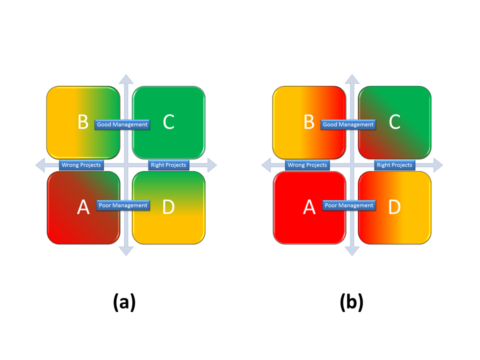
Let’s summarize on a graphic this affirmation. Take a look at Figure 1. On the x axis we can find the presence of appropriate or inappropriate projects in the portfolio and on the y axis the quality of the related project management activities. The graphic can be splitted in four quadrants.

Figure 1.

A - High expense and low income This is clearly the worst situation where one can be. Not appropriate and poorly managed projects. The portfolio suffer from a waste of resources due to poor management activities and from low income due to selection of inadequate projects.

B - Low expense and low income Wrong projects but managed well enough to contain the losses.

C - Low expense and high income This is the best situation. projects accurately selected and managed with reliable processes. 

D - High expense and high income Here the portfolio still suffer from a waste of resources due to poor management activities but it can count on high incomes due to a good projects selection.

It is generally true that everyone’s objective should be to create a portfolio placed in the C quadrant but in times of economic and financial downturn, this may become a matter of pure survival. Please take a look at Figure 2. In part (a), where the weather is fine and the sun shines on your economic situation, you can take the risk to fire some blank cartridges. This is not recommended but there is room for taking additional risks and make some wrong decisions.  when the rain comes in, as depicted in part (b), that it is no more an opportunity and when the mud starts to hit the fan, you are compelled to do better (better projects) with less (better project management). Even a portfolio placed in the quadrant C could not be safe and remunerative enough.

Figure 2.

So how to choose worthy projects to build a portfolio or better, how to choose projects more appropriate for given enterprise environmental factors?

There is a lot in literature about project selection methodologies. In these series of posts I will suggest a method based on some financial considerations. In this and other posts of the series there will be occasional references to statistical elements and concepts. I won’t explain in details each one of them (otherwise I probably would end up with an encyclopedia...) I will provide instead some reference links the first time each concepts is introduced.

Return estimation of a single project

Think of each project like a kind black box. You do not have the slightest idea of what happens inside them, you just know that they absorb resources (money, people, materials...) and that will generate (hopefully) benefits (money, services...).

Return: mean and standard deviation

The first step is to evaluate each project return as the difference of the expected benefits and the required investments, divided by the required investments. All the elements in the ratio should be reconducted to present discounted values. 

Figure 3.

The more you will be able to translate resources and benefits into money, the better you will be able to evaluate the project’s return.

Since the evaluation is based on economic projections and on high level project planning, the best way to do it is to derive a return PDF (Probability Density Function) with the aid of statistical techniques, like Monte Carlo simulations. In Figure 3 is reported an example of return PDF for a fictional project. A PDF is an analytic function that associates to a value on the x axis (in this case the project return) its probability density of occurrence. As an example, according to the return PDF depicted in Figure 3, there is a probability around 8% to achieve a return around 2% from the project. I used the word "around" and not "equal" given the subtle difference between continuous and discrete PDFs.

At this point it is possible, starting from the return PDF, evaluate for each project the mean return value and its standard deviation, that can be directly associated with the estimation uncertainty and with the project’s risk.

In Table 1 depicted in Figure 4 there is a representation of the previous evaluations for some fictional projects.

Figure 4.

Return covariance

The more the covariance of two random variables is great in absolute value, the more these two variables tend to change toghether. That is, if two random variables show great covariance in absolute value, when one of the two variables changes its value, the other one changes it with high probability. If two random variables show small covariance in absolute value, when one of the two variables changes its value, the other one is not bound to change with high probability. If the covariance is equal to zero then the two random variables are independent, that is to say that the behavior of one of them does not influence the other one.

The sign of the covariance shows if two random variables change accordingly. That is, a positive covariance states that two random variables assume great or small values together. A negative covariance states that while one of the two random variables increases (or lessens) its value, the other one lessens (or increases) it. The situation is summarized in Figure 4 Table 2, considering two random variables named x and y. The relationship is symmetric even if, for sake of simplicity, just one part of it is showed.

Assuming the return of each project as a random variable, the estimation of the covariance between each couple of projects is fundamental to properly set up a project portfolio, because it is important to know how the success or the failure of each project could affect the entire portfolio performance. 

Just to make a simple example, if a portfolio contains many projects that show a high degree of positive covariance,  a single project failure could severely affects the performance of the entire portfolio or, vice versa, a single project success could boost the entire portfolio’s return.

In the next post we will see how to select projects that shall be included in a given portfolio given a risk/uncertainty profile, using the statistical concepts here exposed.

Quest' opera è distribuita con licenza Creative Commons Attribuzione - Non commerciale - Non opere derivate 3.0 Unported.

A very simple tool for portfolio analysis

In my post Is it time to go Agile ? I suggested to dispose projects in a bidimensional space, whose coordinates were Innovation and Complexity. This had been done in order to group projects in different classes and to identify for each one the most suitable project management approach.

Figure 1.

In this post I will expand further the concept of projects grouping but with a totally different goal.

The purpose here will be to evaluate reliable indicators to depict the levels of Innovation and Complexity of given portfolios and assess their coherence with the corporate’s profile and business objectives.

To do this we will dive a little in vector’s math to find a more appropriate representation of our bidimensional space.

As it is known a point in a cartesian plane can be unambiguously identified by mean of its two orthogonal projections on the cartesian axes, as shown in Figure 2.

Figure 2

Here the tuple of coordinates (a,b) unambiguously identify the point. This system is called cartesian coordinates system  and numeric values are found on the intersections between  the cartesian axes and the orthogonal lines traced from the given point.

This is not the only possible representation. In Figure 3 is shown the way a point can be unambiguously identified  in the same space by mean of a different set of coordinates. 

Figure 3.

This system is called polar coordinates system and a point is identified by its radius, the point’s distance from the cartesian axes intersection and its azimuth, the angle (positive counterclockwise) from the abscissa axis.

In Figure 3 are also depicted formulas to switch from a coordinates system to the other.

In Figure 4 are shown all possible values for radius and azimuth obtained assigning to Innovation and Complexity values taken from an integer number linear scale ranging from 1 to 6. 

Figure 4.

M (radius) is represented in absolute values while Phi (azimuth) in degrees from 0 to 90.

An overview on values assignement to projects attributes can be found on my post Risk qualitative analysis. How much complicated ?. 

Using polar coordinates the project space represented in Figure 1 looks like as shown in Figure 5.

Figure 5.

Each project is now depicted as a vector and is unambiguously identified by its radius and its azimuth.

An alternative representation for projects in a bidimensional space has been introduced, but was it worth it ? Two numbers we had before (a,b) and two numbers we have now (M, Phi). what is the worth of all this work ?

Figure 6.

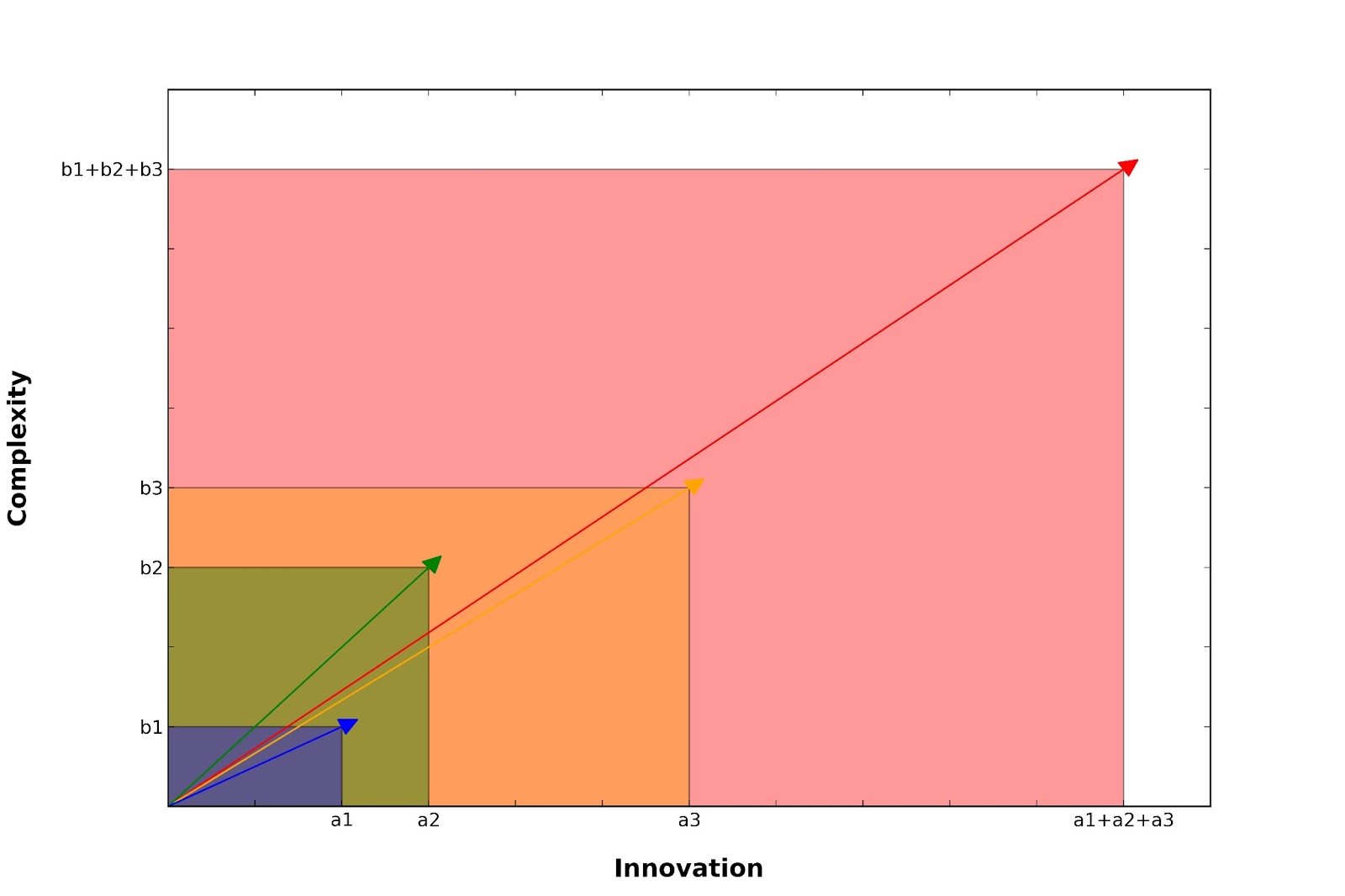
The answer to this question can be found on Figure 6. Observe how the sum operation works on vectors. The sum of N of vectors is still a vector, with abscissa and ordinate equal to the sums of abscissas and ordinates of the N vectors that have been summed together. In this example the red vector is the sum of the blue, yellow and green ones. Consequently the result of this operation depends both on vectors radius and azimuth, as can be observed in Figure 7. 

Figure 7.

Here three vectors with unitary radius are summed together in both the upper and in the lower part of the figure. Vectors in the lower part have a wider range of values for the azimuth coordinate and as a result their summation leads to a vector with a different azimuth and a shorter radius.

So we can say that the more two vectors are alike (radius and azimuth) the more the vector resultant from their summation has a greater radius coordinate. 

As a limit case, if all the 3 vectors in the example were equal in radius and azimuth, the summation result would have been a vector with a radius 3 times the original radius and an azimuth equal to the original one.

Following this line of thought we could add up all the project vectors in the bidimensional space and use the resultant vector as a portfolio indicator. Formulas are depicted in Figure 8.

Figure 8.

The radius value divided by the number of addenda assess how complex is a project in term of Innovation and Complexity, the azimuth how the portfolio is balanced toward the two coordinates. 

A low azimuth indicates that a Portfolio is balanced toward Innovation, a greater one that a Portfolio is balanced toward Complexity. In Figure 9 some examples can be seen. 

Here four portfolios are being analyzed using the suggested indicator. Portfolio in panel a has a lot of projects with an high degree of Complexity and with a medium grade of Innovation. As a result the indicator vector has a great radius and  azimuth values, stating its balance toward Complexity. Portfolio in panel b has some project with an high degree of Complexity and with a medium grade of Innovation and some project with a low degree Complexity and low grade Innovation. As a result the indicator vector has a medium values both for radius and azimuth. There is a balance here between 2 different classes of projects. The bunch of projects near to the ascissa axis counterbalance the high Complexity projects, even if it is clear that the portfolio is still polarized toward Complexity. 

Figure 9.

Portfolio in panels c and d are composed by projects with similar degrees of Complexity and Coherence but with very different balances. The indicator vector here reflects well the situation.

This approach is expandable toward an higher number of dimensions. In case it would support more complex analysis with more parameters, like the Uncertainty parameter proposed as a third dimension in my post “Is it time to go Agile?”. 

Property of Euclidean Space in fact holds for every number of dimensions even if, clearly, our graphical representation capability stops to three. The only price to pay is a little more sophisticated math, since in a K-dimensional space we would have K dimensions to sum together for radius evaluation and K-1 azimuth coordinates.

Quest' opera è distribuita con licenza Creative Commons Attribuzione - Non commerciale - Non opere derivate 3.0 Unported.